3 Nonlinear Retrieval
If the relation of the state  and the corresponding measurement
  (
( ) is
non-linear the replacement in eq. 7 can not be made. We must apply numerical
methods to minimise the cost function. Due to the perculiarities of the Monte
Carlo forward model I must go through the details of the method which was
implemented in McArtimInversion: the Levenberg-Marquardt-Algorithm (LMA).
The LMA is known to be reliable and stable for contineous forward models. It
turned out that LMA can not be used efficiently in combination with a Monte
Carlo forward model due to the statistical noise. It thus needs to be modified to
become efficient.
) is
non-linear the replacement in eq. 7 can not be made. We must apply numerical
methods to minimise the cost function. Due to the perculiarities of the Monte
Carlo forward model I must go through the details of the method which was
implemented in McArtimInversion: the Levenberg-Marquardt-Algorithm (LMA).
The LMA is known to be reliable and stable for contineous forward models. It
turned out that LMA can not be used efficiently in combination with a Monte
Carlo forward model due to the statistical noise. It thus needs to be modified to
become efficient.
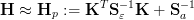
3.1 Gauss-Newton Method
A simple algorithm is the Gauss-Newton method. It is the Newton method
which iteratively calculates the roots of a function g(x) and it is applied to
the gradient of the cost function. The well known ’1D’ iteration formula
is
![xi+1 = xi - [g′(xi)]-1yi.](Inversion52x.png) | (12) |
The relation is obtained by the considerations depicted in fig. ??. Here, the ’half’
gradient of the cost function is used for the function g(x):
![⃗g(⃗x) = KT S-ɛ1[⃗F(⃗x ) - ⃗y] + S-a 1[⃗x - ⃗xa]](Inversion53x.png) | (13) |
The iteration procedure in equation 12 is formally the same:
![- 1
⃗xi+1 = ⃗xi - [⃗∇ ⃗g(⃗xi)] ⃗g(⃗xi)](Inversion54x.png) | (14) |
A closer look on g′(x) yields:
![H := ⃗∇⃗g(⃗x) = ⃗∇KT S-ɛ 1[⃗F (⃗x) - ⃗y] + KT S -ɛ1K + S-a 1.](Inversion55x.png) | (15) |
The first summand is usually ommited in high dimensional problems, because a)
it can be neglected near the optimum if the forward model is able to approximate
the forward function adequately and b) it is computionally expensive and
complicated to calculate (tensor of third order). 
 (
( ) is hence approximated
by
) is hence approximated
by
 | (16) |
Formally 
 (
( ) is the Hessian of the cost function χ2(
 ). The simplification
made in eq. 16 is therefor sometimes called Pseudo-Hessian approach. In
total, the Gauss-Newton iteration procedure for our class of problems
is:
). The simplification
made in eq. 16 is therefor sometimes called Pseudo-Hessian approach. In
total, the Gauss-Newton iteration procedure for our class of problems
is:
![[ T -1 -1]-1{ T - 1 ⃗ - 1 }
⃗xi+1 = ⃗xi + K i S ɛ Ki + S a K i Sɛ [⃗y - F (⃗xi)] - Sa [⃗xi - ⃗xa]](Inversion64x.png) | (17) |
The Gauss Newton method converges rapidly close to the optimum, i.e. when the
gradient of the cost function is linear, resp. when χ2 can be approximated by a
2nd order polynomial.
3.2 Levenberg-Marquardt Method
There are situations in which the Gauss-Newton method diverges. To face these
problems Levenberg [Levenberg 1944] suggested to modify the Newton
method by introducing an additional summand in the (Pseudo) Hessian
Hp:
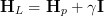 | (18) |
where I is the N × N unity matrix. Instead of eq. 18 Donald Marquardt [D.
Marquardt 1963] suggested to use
 | (19) |
The whole iteration scheme is then
![[ - 1 T -1 ]-1{ T -1 -1 }
⃗xi+1 = ⃗xi + (1 + γi)Sa + K i S ɛ Ki K i Sɛ [⃗y - ⃗F (⃗xi)] - Sa [⃗xi - ⃗xa]](Inversion67x.png) | (20) |
and can be explained as follows. Alltogether, the Levenberg-Marqardt algorithm is
an intelligent combination of the steepest descent and the Gauss-Newton
method. Depending on the local situation the mixture is controlled by the
parameter γ. If the gradient is strongly non-linear, γ should be increased. For
very huge γ the method tends to the (slow but stable) steepest descent
method:
![γ≫1 1 { T -1 -1 }
⃗xi+1 = ⃗xi + --Sa K i S ɛ [⃗y - ⃗F(⃗xi)] - S a [⃗xi - ⃗xa ]
γi ◟---------------◝◜----------------◞
-⃗g(⃗xi)](Inversion68x.png) | (21) |
because  (
( ) is the gradient of the cost function at the position
  . If the
  (
( )
is approximately linear, γ may be decreased such that the method is
more like the Gauss-Newton method (compare to eq. 17). The iteration
should be stopped if a certain convergence criterium is met. Rodgers
proposed:
)
is approximately linear, γ may be decreased such that the method is
more like the Gauss-Newton method (compare to eq. 17). The iteration
should be stopped if a certain convergence criterium is met. Rodgers
proposed:
![[F⃗(⃗xi+1) - ⃗F(⃗xi)]TS- 1[⃗F (⃗xi+1) - F⃗(⃗xi)] ≪ M
δˆy](Inversion74x.png) | (22) |
with the δŷ covariance matrix:
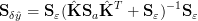 | (23) |
3.2.1 Iteration Scheme and a Strategy to Adjust γ
We will now discuss how the equations above are used in a common LMA
implementation, to find the minimum of a cost function χ2( ). The procedure is
as follows:
). The procedure is
as follows:
- Find a good estimate
 0 of the optimum. This can be done by heuristic
assumptions about the state or even by taking the a priori
0 of the optimum. This can be done by heuristic
assumptions about the state or even by taking the a priori  a, choose
γ1. Calculate χ2(
a, choose
γ1. Calculate χ2( 0)
0)
- Apply eq. 20 to find
 trial
trial
- Check χ2(
 trial) < χ2(
 i). If
- yes: check eq. 22, If
- yes: found optimal state
 =
=  trial
trial
- no: set
 i+1 =
i+1 =  trial and go to 2.
- no: adjust γ and recalculate
 trial, go to 3.
There are several possible strategies to adjust the parameter γ. The simpliest method
is to increase γ by a factor of 2 to 10 and therewith refine the step size in
step ’3-no’ until a state is found which minimises the cost function. This
strategy should work in any case because the larger γ is, the closer the state
will be situated along the steepest descent direction. If a valid state is
found γ can be decreased again (by a factor of, say 3). With this simple
procedure it is assured, that in each iteration a state is found which minimises
χ2.
3.3 Total State Vector
Combining the retrieval of trace gases using DOAS SCDs and intensities or O4
SCDs (O4 method described in [Wagner 2004], technical details in [Friess et al.
2006]) has benefits in comparison with the separate retrievals, provided that a
priori knowledge or other constraints with respect to the trace gas is
present. The reason is simply, that the aerosol properties, as they influence
the trace gas SCD have to be consistent with the a priori knowledge of
the trace gas. In such a combined retrieval, the state vector is denoted
by
 | (24) |
and the measurement vector is
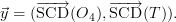 | (25) |
Accordingly, the K matrix is given by
 | (26) |
3.4 “Secure State Vector Transformations
The iterative algorithm proposed here is not sensitive to the physical meaning of
the state vector, i.e. it does not know, that e.g. a concentration has to be positive.
It hence may happen, that a proposed state  trial is physically invalid. Even in the
linear retrieval, the result could be a negative concentration. Similarely,
the single scattering albedo has to be in ϖ0
trial is physically invalid. Even in the
linear retrieval, the result could be a negative concentration. Similarely,
the single scattering albedo has to be in ϖ0  (0, 1] and the asymmetry
parameter g (-1, 1). To avoid that the algorithm accidentally yields
an unphysical state vector, the state vector is transformed into a secure
form
for which the problem does not exist.
(0, 1] and the asymmetry
parameter g (-1, 1). To avoid that the algorithm accidentally yields
an unphysical state vector, the state vector is transformed into a secure
form
for which the problem does not exist.
The transformation of the state vector component a to its secure form ξa is
denoted by
 | (27) |
Consequently, K is transformed to Ξ:
 | (28) |
So the Jacobian of  with respect to the secure state vector
  x of
x of  is obtained
from K by multiplying the element of K with ∂s∕∂ξxj. For example, a “secure
transformation of aerosol extinction coefficients and trace gas number densities x
is
is obtained
from K by multiplying the element of K with ∂s∕∂ξxj. For example, a “secure
transformation of aerosol extinction coefficients and trace gas number densities x
is
 | (29) |
and the Ξ matrix is
 | (30) |
The other secure transformations and their jacobians are listed in the following
table 1.
| Table 1: | Secure transformations of state vector components aerosol
extinction coefficient and trace gas number densities ɛ, aerosol single
scattering albedo ϖ0 and aerosol phase function asymmetry parameter g. |
|
3.5 LMA with a Monte Carlo Forward Model
The Levenberg-Marquardt algorithm implicitely assumes that the forward model
which is used to calculate  (
( ) and the K-matrix is contineous in
  . Especially in
step 3 of the iteration scheme, this property is required to be able to compare the
cost function evaluated at two different states. In combination with a Monte Carlo
forward model, the user will encounter difficulties in step 3, because the stochastic
noise will disturb the comparison: If γ is increased, the test state
. Especially in
step 3 of the iteration scheme, this property is required to be able to compare the
cost function evaluated at two different states. In combination with a Monte Carlo
forward model, the user will encounter difficulties in step 3, because the stochastic
noise will disturb the comparison: If γ is increased, the test state  trial will be in a
closer environment of the last valid state and unfortunately, the change of
trial will be in a
closer environment of the last valid state and unfortunately, the change of
 (
( trial) with respect to
  (
( i) will be less distinguishable from the Monte
Carlo noise. Hence it is required, that the MC-error is controlled by an
additional mechanism. To get an effective method, the local situation
needs to be investigated and a criterium, that indicates whether a better
accuracy of the quantities
i) will be less distinguishable from the Monte
Carlo noise. Hence it is required, that the MC-error is controlled by an
additional mechanism. To get an effective method, the local situation
needs to be investigated and a criterium, that indicates whether a better
accuracy of the quantities  (
( ) and K respectively is really needed, has to be
developed.
) and K respectively is really needed, has to be
developed.
The error of χ2 in eq. 4 induced by the Monte Carlo noise is
![|| 2 || | |
Δ χ2 (⃗x) = ||∂χ-(⃗x)-Δ ⃗F (⃗x )||= 2 ||Δ F⃗T (⃗x )S-1[⃗F (⃗x ) - ⃗y]||
MC | ∂ ⃗F MC | MC ɛ](Inversion119x.png) | (31) |
On the opposite side and by an analogous calculation the error of χ2 due to the
measurement error is obtained:
![2 || T -1 ||
Δɛχ (⃗x ) = 2|⃗σɛ S ɛ [⃗F(⃗x) - ⃗y]|.](Inversion120x.png) | (32) |
In principle the algorithm is allowed to keep ΔMCχ2( ) > Δ
ɛχ2(
) > Δ
ɛχ2( ), if it is
permitted by the situation. Then the χ2 accuracy does not need to be increased if
ΔMCχ2(
), if it is
permitted by the situation. Then the χ2 accuracy does not need to be increased if
ΔMCχ2( ) < Δ
ɛχ2(
) < Δ
ɛχ2( ). The number of quadrature trajectories is increased only
if
). The number of quadrature trajectories is increased only
if
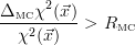 | (33) |
where RMC is a user defined threshold. Another possibility to deal with the
aforementioned problems is to apply the dependent sampling MC technique. A
single trajectory ensemble is used to perform step 3 of the iteration scheme for all
γ. With the dependent sampling technique the χ2 becomes contineous and the
normal scheme works.

 +
+  arctan (
 cos
cos  ))
)) ))
)) arctan (
 cos
cos  )
) 