In the case of a linear forward function (approximated by a linear forward model), one may write
|
| (7) |
The minimisation problem then is:
![KT S-ɛ1[K ⃗x - ⃗y] + S -a1[⃗x - ⃗xa] = 0](Inversion38x.png) | (8) |
and is readily solved for  :
:
![T -1 - 1-1 T -1 -1
ˆx = [K S ɛ K + Sa ] [K S ɛ ⃗y + Sa ⃗xa].](Inversion40x.png) | (9) |
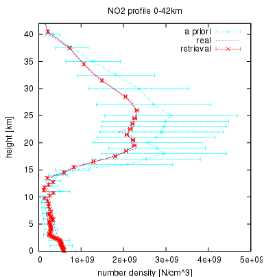
To demonstrate the method, the linear retrieval of a NO2 vertical profile performed using simulated data (fig. 2.1). The measurement vector consists of NO2 SCD’s which would be measured during the ascent of a ballon with an instrument looking horizontally into the layer of the ballon height. The forward model was used to simulate the measurement. Then the profile was altered and the inversion scheme was tested using the altered profile as a priori input. As shown in the figure, the algorithm reproduces the real profile which was used to simulate the measurement. If the tropospheric region is magnified, it is observed that the algorithm tends to return the a priori profile information in regions where the overlap of the real profile and the a priori expectation is small.
For a sensitivity analysis, two questions may be asked: How much does the result
 depend on the a priori state and on the real state of the atmosphere? The
former part of the question is answered by the derivative
depend on the a priori state and on the real state of the atmosphere? The
former part of the question is answered by the derivative
![∂xˆ-= [KT S -1K + S-1]-1S- 1
∂⃗xa ɛ a a](Inversion44x.png) | (10) |
The trace of the resulting matrix provides the number of parameters which are
introduced by the a priori state vector. It is eligible, that this number tends to
zero. Vice versa, and answering the latter question the averaging kernel matrix is
obtained by assuming  = K
= K real in eq. 9
![∂ ˆx
----- = [KT S -ɛ1K + S-a1]-1KT S -ɛ1K
∂ ⃗xreal](Inversion47x.png) | (11) |
The trace of the averaging kernel matrix quantifies the information content of
the measurement and is the number of components of  which could be
retrieved independently from the a priori state. A more detailed discussion
on averaging kernels and information content can be found in [Rodgers
2000].
which could be
retrieved independently from the a priori state. A more detailed discussion
on averaging kernels and information content can be found in [Rodgers
2000].