1 Introduction
Consider a physical process or system which can be described roughly by a finite
set of parameters  and
and  , such as the radiative transfer in the atmosphere and
the optical properties in disjunct layers of the atmosphere confined into the
vectors
, such as the radiative transfer in the atmosphere and
the optical properties in disjunct layers of the atmosphere confined into the
vectors  and
and  . We distinguish between parameters of interest
  and those
  which are required to describe “the rest” of the system. The vector
  is called
state and shall be obtained by measurements. Sometimes there is prior
knowledge about the state. Then an expectation
is called
state and shall be obtained by measurements. Sometimes there is prior
knowledge about the state. Then an expectation  a (’a’ stands for a priori)
and a standard deviation
a (’a’ stands for a priori)
and a standard deviation  a which quantifies the natural variability of
  (climatology) is given. Using an adequate instrument, the outcome of
the measurements will be dominated by the physics of the process. One
writes
(climatology) is given. Using an adequate instrument, the outcome of
the measurements will be dominated by the physics of the process. One
writes
 | (1) |
where  is the measurement vector with the measurement values as components
and
is the measurement vector with the measurement values as components
and  is the forward function which symbolises the physics of the process.
In reality
is the forward function which symbolises the physics of the process.
In reality  often also depends on parameters of the instrument but for
the present considerations it is assumed to have a perfect instrument.
Besides
often also depends on parameters of the instrument but for
the present considerations it is assumed to have a perfect instrument.
Besides  , a vector
  ɛ is obtained, which is the standard deviation of
 .
.
1.1 Forward Model
In order to infer parts of the state from measurements the physics of the process  has to be understood. In detail,
  in eq. 1 has to be approximated by a forward
model
in eq. 1 has to be approximated by a forward
model  :
:
 | (2) |
The forward model should be able to simulate the outcome of the measurement at
least with an accuracy better than the measurement error. In the following, the
dependence of the forward model on the parameters  is ommitted in the notation
and
is ommitted in the notation
and  (
( ) is used instead. But it is emphasized, that knowledge of
  is needed to
model the process correctly.
is needed to
model the process correctly.
1.2 Cost Function
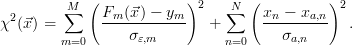
Assume that M measurements have been made and the state to be retrieved has
N components. The cost function χ2( ) is a measure of the deviation of
the simulated measurement from the real measurement and is defined
as
) is a measure of the deviation of
the simulated measurement from the real measurement and is defined
as
 | (3) |
To reflect the accuracy of the measurement respectively the prior knowledge each
summand is divided by the corresponding standard deviation σ. The inverse
problem is then a χ2-optimisation problem, i.e. a state  that minimises the cost
function has to be found. If the a priori profile is considered, the resulting state is
the best (optimal) compromise between the a priori knowledge and the
measurement. But as will be seen later in an example the a priori information is
only used where it is needed.
that minimises the cost
function has to be found. If the a priori profile is considered, the resulting state is
the best (optimal) compromise between the a priori knowledge and the
measurement. But as will be seen later in an example the a priori information is
only used where it is needed.
It is expedient to rewrite the cost function in a more compact form:
![χ2(⃗x) = [⃗F(⃗x ) - ⃗y]TS -ɛ1[⃗F(⃗x) - ⃗y] + [⃗x - ⃗xa ]TS -a1[⃗x - ⃗xa].](Inversion28x.png) | (4) |
The measurement covariance (M × M) and a priori covariance (N × N)
matrices contain the squares of the standard deviations  ɛ and
ɛ and  a on the
diagonal:
a on the
diagonal:
 | (5) |
When the off-diagonal elements are filled with zeros than eqs. 3 and 4
are formally equal. There exists a class of inversion methods which fill
the off-diagonal elements with non-zero values in order to get a smooth
result (regularisation). The criterium which  has to fullfill to minimise
the cost function, i.e. to fit the simulated
has to fullfill to minimise
the cost function, i.e. to fit the simulated  (
( ) to the measurement
  is
is
![⃗∇ χ2(ˆx) = 0 i.e. ⃗∇F⃗(⃗x)T S-1[⃗F (⃗x ) - ⃗y] + S- 1[⃗x - ⃗x ] = 0
ɛ a a](Inversion36x.png) | (6) |
Depending on the nature of the relation eq. 1 there are two groups of inversion
schemes: linear one-step and non-linear iterative retrievals.