4 Application of the Program McArtimInversion

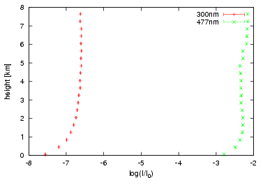
In order to demonstrate the capabilities of the non linear inversion procedure in combination with a MC RTM this section discusses the retrieval of an aerosol profile from a simulated measurement which consists of logarithmic sun normalised radiances log (I∕I₀) at 300nm and 470nm recorded in different heights. For both wavelength aerosol parameters ϖ₀ = 1 and g = 0.67 has been chosen and the ground albedo was set to 0.05. The geometry description file is listed in figure 2.

The height definition in line 1 is ignored, since it is overwritten in the simulation script (file content listed in Fig. 3).

The resulting logarithmic intensities are plotted in the left panel of figure 4

Figure 4: Top-left: Simulated logarithmic sun normalised radiances. Top-right: effective number of scatter events for ground, Rayleigh and aerosol scattering, where the aerosol phase function was approximated by the Henyey-Greenstein model with g = 0.67. Bottom panels: profile evolution during the non linear inversion at 300nm (left) and 477nm (right).

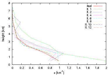
In principle, it should be possible to invert the aerosol profile from the 21 measurements, so the a priori information was not considered and it has beed tried to retrieve the profile from the measurement only. The cost function was

(34)

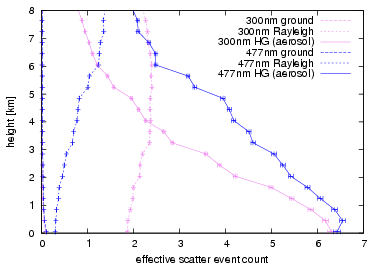
Figure 4 shows the profile evolution in different steps of the iteration. The difference of the RT at 300nm and 477nm is the ratio of the Rayleigh extinction coefficient ɛ_R to the aerosol extinction coefficient ɛ_A. This can be seen cleary from the top-right panel of Fig. 4: at 300nm and above 4km ɛ_A is smaller than ɛ_R, where at 477nm ɛ_A is always greater than ɛ_R. In consequence, the 477nm measurement is generally more sensitive towards the presence of an aerosol.